David Wessel, Cyril Drame, and Mathew Wright ({wessel, cyril, matt}@cnmat.berkeley.edu)
Center for New Music and Audio Technologies (CNMAT), 1750 Arch Street, Berkeley, CA 94709

Control oriented implementations of neural network models and memory-based models are developed and compared. These techniques model the spectral data from instruments as opposed to the physical sound production mechanism. Both model types are for real-time control and use controller inputs such as pitch, loudness, and brightness functions to produce frequencies and amplitudes for sinusoidal components in an additive synthesizer. Both approaches produce acceptable synthesis results. Network models are compact but inflexible as the data is discarded after learning. Memory models are more memory intensive and maintain the data for local reference. Experiments with wind instruments and singing voice are presented.

Analysis-synthesis methods have for the most part privileged time warping and pitch shifting. Musical signals analyzed by such methods as the phase vocoder and sinusoidal modeling allow composers to stretch and shrink the time axis independent of the pitch and to alter the pitch without altering the duration. These time and pitch modifications have been put to practical and creative use, but the fact that the time-stretched sounds preserve the order of the evolution of the sound’s spectral features greatly constrains the nature of the potential transformations. The data from such analysis methods does not afford the construction of new phrases, this is to say, new sequences of pitches and amplitudes. An additional form of abstraction is required to escape the contiguous structure inherent in the data provided by the majority of the available analysis methods. In this paper we explore two approaches inspired by control theory that remove the temporal axis from the analysis data and provide synthesis models that can be played with envelope functions.

We begin with a set of data obtained from the sinusoidal analysis of an extended monody played by a nearly-harmonic musical source like a voice, wind, or string instrument. We assume the data to be organized in time-tagged frames, like those specified in the Sound Description Interchange Format (http://www.cnmat.berkeley.edu/SDIF), containing frequencies, amplitudes, and phases of the nearly-harmonic components. We further assume that they are sufficient for an accurate resynthesis. Our goal is to obtain a model of the analyzed instrument so we can play a new melodic figure on it by supplying new pitch and loudness envelope functions. Towards this goal, we estimate the values of the control functions corresponding to our analyzed phrase. We will likely have good pitch estimates already as they often play a role in the spectral estimation process. We obtain a loudness estimate by applying a loudness summation model like those proposed by Zwicker and Scharf , and Moore and Glasberg .

As illustrated in Figure 1, we now have pitch and loudness as controllers and the frequencies, amplitudes, and phases of a number of sinusoids as outputs of a model, a model we must somehow determine.

Figure 1: Our model is a "black box" mapping control parameters to spectral detail

In this section we describe two contrasting approaches to model specification: a multi-layer neural network supervised learning approach and a memory-based model that reorganizes the spectral frames in a matrix indexed by pitch and loudness or whatever the controllers have been selected to be.

A neural network is a parametric model. The network is a function with a finite set of parameters. The learning process, in our case back-propagation learning, fits the function to all of the data by estimating the parameters. The fitted network is used as the instrument model and the training data are discarded.

By contrast, memory based models are non-parametric. The number of parameters varies with the amount of data. The data is not fit once and for all and discarded, but is kept for reference in what are usually very local computations. While the networks globally fit the data, the memory models combine local examplars determined by the input functions.

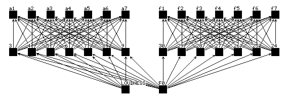
A neural-network model is illustrated in Figure 2. The input units accept the pitch and loudness functions and the output units produce the frequencies and amplitudes of the sinusoidal components for the additive model. We will leave the phases out of the picture for the moment, acknowledging that they are perceptually relevant , but inseparable from the frequencies estimated by our analysis methods and produced by our additive synthesizer.

Figure 2: A neural network architecture for sound modeling. The input layer receives loudness and pitch (F0) functions. The output layer produces partial amplitudes and frequency values. The networks we used in practice had upwards to 80 hidden and output units.

In the experiments that we report here we trained the networks with a back-propagation learning method. One of the important features of our training method is the use of an error norm or cost function based on a perceptual model. Rather than use a brute minimum-squared-error approach to produce an overall error from the differences between the model’s amplitude estimates and the original amplitudes, we weigh the contribution of each difference as a function of frequency. We weigh the amplitude fit error more heavily in the spectral regions where the ear is most sensitive. The errors for the frequency estimates are treated uniformly throughout.

The actual networks we designed for modeling were more complicated than the model we have just described. We have experimented with extending the input units backward over a number of frames in an effort to capture state in the instrument. We have added a set of muting output units on the amplitude units so that when the loudness is at zero all the output amplitudes are shunted to zero.

We implemented a non-parametric model for generating spectral data from controllers. The memory-based approach uses a subset of the original data set to generate the outputs corresponding to each input value. This corresponds to local function fitting; it does not model all data simultaneously. This type of model has to memorize all data and is therefore called memory-based.

We used the same database as the one used for the neural network technique: We stored every set of inputs and their corresponding outputs in two matrices, namely X and Y. Each row X_i of the X matrix contains an input vector [F0, loudness, ...]. Each row Y_i of the Y matrix contains the corresponding output vector, a spectral frame.

For each new input x(q) [F0_requested, loudness_requested] we first calculate the distance from each of the stored data points:

n: number of control inputs

The factor s(j) reflects a positive weighting (distance metric) among the n input dimensions, either to normalize them or to give them different importance.

Then we choose the k closest neighbors in the inputs space according to this distance, and we calculate a weight as a function of the distance for each of those k stored data points. We used a Gaussian Kernel:

The parameter c scales the size of the kernel. Together with parameter k it determines how local the model will be.

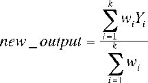
The new output vector is finally computed by weighted average of each of the corresponding k selected outputs:

In this section we give an overview of some experiments we performed using both techniques and briefly present some of our results.

This set of experiments demonstrates that the models described in the previous section not only can successfully capture the global spectral behavior of a specific instrument, but can also provide good control over some of its fine timbral characteristics.

We used a three-dimensional input space where the dimensions were pitch, loudness, and brightness. We obtain a measure of brightness by computing the centroid for each spectral frame.

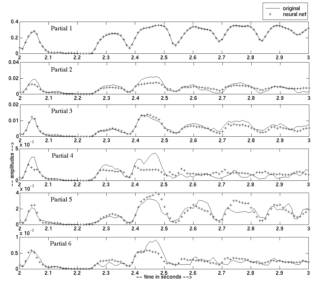
A one-second portion of results, showing how well the neural network model does when asked to replay the suling data it was trained on, is displayed in Figure 3. The original phrase is about 10 seconds long. Keep in mind that the scale of each graph is magnified as the partial number increases. We also obtained very good results on the saxophone database where we used 30 partials.

We generally obtained perceptually satisfying results when we presented new sets of inputs to our model. For instance we presented the inputs of the suling phrase to the saxophone models and vice-versa. The results are pretty convincing although up to date, the neural network model seems to exhibit better aptitudes for generalization. Global timbral instrument behaviors are successfully captured. By changing only the value of the brightness input, we are able to control brightness in real time.

Additional experiments with vocal sounds and an extensive set of viola glissandi yielded good results. In all of the preliminary experiments only sinusoids at nearly harmonic frequencies were used. The residual aspects of the spectral models are yet to be controlled with these techniques and we expect considerable improvement in the synthesis when they are integrated into the models.

Both the neural-network and memory based models functioned well in a real-time context. It would seem that the non-parametric character of the memory-based models make them more flexible, easier to modify, and more adapted to creative musical use. The network models, on the other hand, are very compact and appear to generalize well. In general the network models provided a smoother sounding result than the memory-based models.

Figure 3: Comparison between real Suling amplitudes and Neural Net outputs

References