Center for New Music and Audio Technologies

The CORDIC-Algorithm for Computing a Sine

In 1959 Jack E. Volder [7] described the COordinate Rotation DIgital Computer or CORDIC for the calculation of trigonometric functions, multiplication, division and conversion between binary and mixed radix number systems. The CORDIC-algorithm provides an iterative method of performing vector rotations by arbitrary angles using only shifts and adds. Volder's algorithm is derived from the general equations for vector rotation. If a vector $V$ with components $(x,y)$ is to be rotated through an angle $\phi$ a new vector $V'$ with components $(x',y')$ is formed by:

$$V'=\left[\begin{array}{c} x'\\ y'\end{array}\right]=\left[\begin... ...s(\phi)-y\cdot\sin(\phi)\\ y\cdot\cos(\phi)+x\cdot\sin(\phi)\end{array}\right]$$ (1.2)

Figure 1.2 illustrates the rotation of a vector $V=\left[\begin{array}{c}x\\ y\end{array}\right]$by the angle $\phi$.

Figure 1.2: Rotation of a vector V by the angle $\phi$

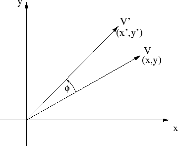The individual equations for $x'$ and $y'$ can be rewritten as [8]:

$$x' = x\cdot\cos(\phi)-y\cdot\sin(\phi)$$ (1.3)

$$y' = y\cdot\cos(\phi)+x\cdot\sin(\phi)$$ (1.4)

and rearranged so that:

$$x' = \cos(\phi)\left[x-y\cdot\tan(\phi)\right]$$ (1.5)

$$y' = \cos(\phi)\left[y+x\cdot\tan(\phi)\right]$$ (1.6)

The multiplication by the tangent term can be avoided if the rotation angles and therefore $\tan(\phi)$ are restricted so that $\tan(\phi)=2^{-i}$. In digital hardware this denotes a simple shift operation. Furthermore, if those rotations are performed iteratively and in both directions every value of $\tan(\phi)$ is representable. With $\phi=\arctan\left(2^{-i}\right)$ the cosine term could also be simplified and since $\cos(\phi)=\cos(-\phi)$ it is a constant for a fixed number of iterations. This iterative rotation can now be expressed as:

$$x_{i+1} = K_i\left[x_i-y_i\cdot d_i\cdot 2^{-i}\right]$$ (1.7)

$$y_{i+1} = K_i\left[y_i+x_i\cdot d_i\cdot 2^{-i}\right]$$ (1.8)

where $K_i=\cos\left(\arctan\left(2^{-i}\right)\right)$ and $d_i=\pm1$. The product of the $K_i$'s represents the so-called K factor [9]:

$$K=\prod_{i=0}^{n-1}K_i\;.$$ (1.9)

This $K$ factor can be calculated in advance and applied elsewhere in the system. A good way to implement the $K$ factor is to initialize the iterative rotation with a vector of length $\vert K\vert$ which compensates the gain inherent in the CORDIC algorithm. The resulting vector $V'$ is the unit vector as shown in Figure 1.3.

Figure 1.3: Iterative vector rotation, initialized with V0

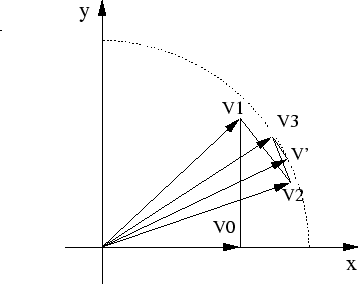Equations 1.7 and 1.8 can now be simplified to the basic CORDIC-equations:

$$x_{i+1} = \left[x_i-y_i\cdot d_i\cdot 2^{-i}\right]$$ (1.10)

$$y_{i+1} = \left[y_i+x_i\cdot d_i\cdot 2^{-i}\right]$$ (1.11)

The direction of each rotation is defined by $d_i$ and the sequence of all $d_i$'s determines the final vector. This yields to a third equation which acts like an angle accumulator and keeps track of the angle already rotated. Each vector $V$ can be described by either the vector length and angle or by its coordinates $x$ and $y$. Following this incident, the CORDIC algorithm knows two ways of determining the direction of rotation: the rotation mode and the vectoring mode. Both methods initialize the angle accumulator with the desired angle $z_0$. The rotation mode, determines the right sequence as the angle accumulator approaches 0 while the vectoring mode minimizes the y component of the input vector^1.2.

The angle accumulator is defined by:

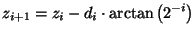$$z_{i+1}=z_i-d_i\cdot\arctan\left(2^{-i}\right)$$ (1.12)

where the sum of an infinit number of iterative rotation angles equals the input angle $\phi$ [10]:

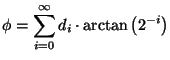$$\phi=\sum_{i=0}^{\infty}d_i\cdot \arctan\left(2^{-i}\right)$$ (1.13)

Those values of $\arctan\left(2^{-i}\right)$ can be stored in a small lookup table or hardwired depending on the way of implementation. Since the decision is which direction to rotate instead of whether to rotate or not, $d_i$ is sensitive to the sign of $z_i$. Therefore $d_i$ can be described as:

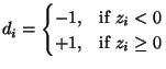$$d_{i}= \begin{cases}-1, &\text{if $z_{i} < 0$}\\ +1, &\text{if $z_{i} \geq 0$} \end{cases}$$ (1.14)

With equation 1.14 the CORDIC algorithm in rotation mode is described completely. Note, that the CORDIC method as described performs rotations only within $-\pi/2$ and $\pi/2$. This limitation comes from the use of $2^0$ for the tangent in the first iteration. However, since a sine wave is symmetric from quadrant to quadrant, every sine value from 0 to $2\pi$ can be represented by reflecting and/or inverting the first quadrant appropriately.

Home